Andrew B.

Recycle Sorting Robot With Machine Learning & Robotic Arm

Did you know that the average contamination rate in communities and businesses range up to 25%? That means one out of every four pieces of recycling you throw away doesn’t get recycled. This is caused due to human error in recycling centers. Traditionally, workers will sort through trash into different bins depending on the material. Humans are bound to make errors and end up not sorting the trash properly, leading to contamination. As pollution and climate change become even more significant in today’s society, recycling takes a huge part in protecting our planet. By using robots to sort through trash, contamination rates will decrease drastically, not to mention a lot cheaper and more sustainable. To solve this, I created a recycle sorting robot that uses machine learning to sort between different recycle materials.

Engineer	School	Area of Interest	Grade
Andrew B.	Palo Alto High School	Aerospace Engineering	Incoming Junior

REFLECTION

My experience at Bluestamp was fantastic. I always loved to build things at home. Bluestamp is an environment filled with students and instructors that share my passion for building and learning new things specifically in engineering. This was a super unique experience that I would not be able to experience at my high school.

DEMO VIDEO

DEMO NIGHT PRESENTATION

FINAL MILESTONE

Today I completed my final milestone which was to mount all the components into a project box, enable the Edge TPU’s maximum frequency, and to make the robotic arm more accurate.

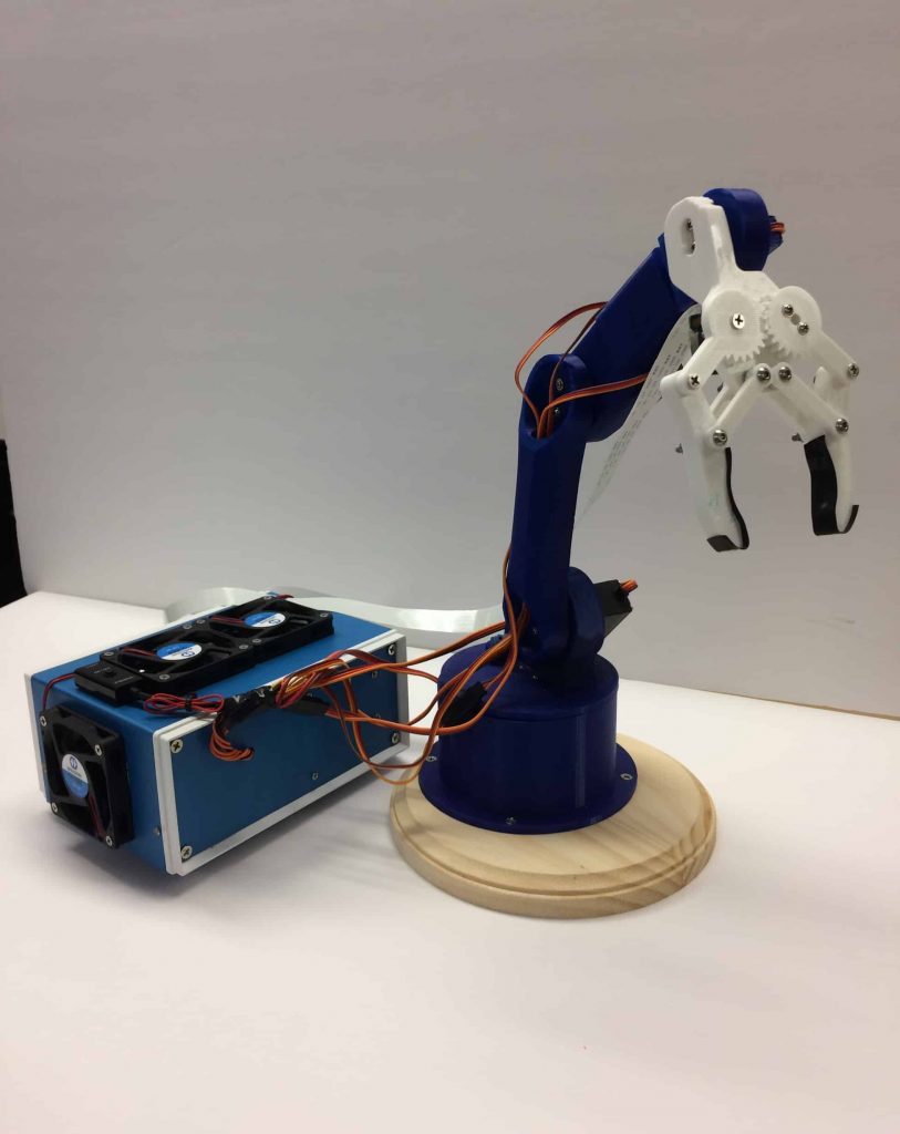
I decided to use an aluminum project box that had sufficient space to fit the Arduino, Raspberry Pi, and the Coral Edge TPU USB Accelerator. Aluminum is great because it acts like a huge heat sink for my components. In order to mount all the hardware in the project box, I used brass standoffs to better help cool the components. The RPI and TPU would reach extremely high temperatures.

These components process the object detection and thus are under a lot of computation load. When the RPI operated outside of the case, it still achieved high temperature levels. I decided to add four fans for active cooling to complement passive cooling from the heat sinks.

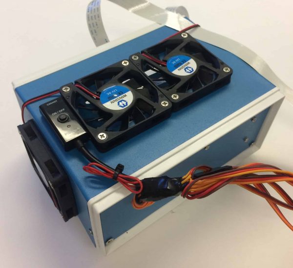
Now, I have passive and active cooling to help cool all my components. The four fans all run on 12 volts, so I had to add an extra power supply and solder all the fan wires into a bullet connector for my power supply. With the fans on the RPI did not run hot when running object detection. Usually, it reached high enough temperatures to burn your skin to the touch. With the fans, it ran casually warm. Below is a picture of all my components inside the aluminum project box.

After mounting all the components in a project box with fans, I was also able to reach the maximum frequency the Coral Edge TPU can operate at. When installing the edgetpu API, there is a feature to enable the setting to make the TPU run at a higher frequency than default. This will allow for better frames per second than if running the TPU at a lower frequency. Using this feature, I get one more frame faster than before. I achieved an average of 15.5 fps which is better than my previous 14.5 fps using the default frequency. I also was able to make my robotic arm more accurate.

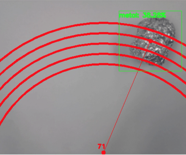
This was done by adding more distance presets. As explained during my Third Milestone, I used distance presets to pick up the detected object based on how far it was from my robotic arm. By adding more, it would become even more precise and accurate. Below is an image showing more preset circles from the video feed.

I would still like to add more modifications to my project. For example, I’m thinking of adding a relay switch to automatically turn on and off the cooling fans based on how hot the CPU was. If the CPU passes a certain temperature, the RPI will send a signal to the relay to switch the cooling fans on. This would prevent wearing out the cooling fans because they will only turn on when needed.

Finally, I’m super excited I successfully completed my project in a short period of time.

screen-shot-2019-07-19-at-3.58.27-pm-600x500

THIRD MILESTONE

Today, I completed my third milestone which was to connect my Raspberry Pi to my Arduino using USB-to-Serial communication so my robotic arm can pick up the recognized piece of recycling and drop it according to its material type.

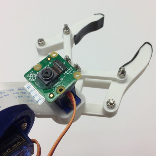
The first step was to mount my RPI camera to my robotic arm so that it can perform object detection. This was done by simply hot gluing the camera to the bottom of my clamping servo of the robotic arm. When the robotic arm is in its default or home position, the camera will be facing directly below the robotic arm. Below is a picture of my camera mounted on my robotic arm.

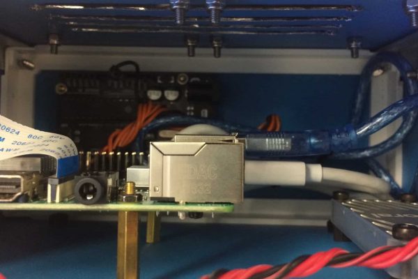
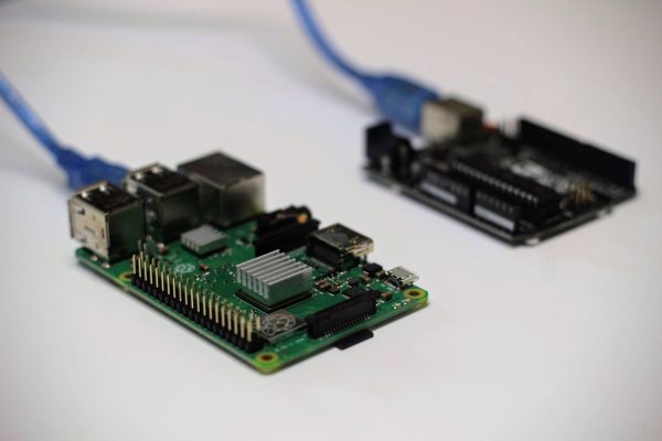
Next, I had to connect the Arduino and RPI together via a USB cable in order to perform USB-to-Serial communication. The image below shows how I connected my RPI to my Arduino. I reprogrammed the RPI and Arduino to enable communication between each other. On the Arduino, this can easily be done using the built-in Serial functions, like Serial.begin(). This starts serial communication from the USB. Being able to test the Arduino’s serial communication was made easy due to the Arduino IDE’s serial monitor. You can receive and send data via serial communication. By replicating data signals that would come from the RPI, I was able to quickly debug and program the robotic arm.

To program the robotic arm, I assigned variables to store values coming from the RPI. These included the type of material it detected, it’s distance, and which angle the base servo motor needs to turn. With this information, I simply created functions that essentially take the data from the RPI and pick up the object. I experienced many issues trying to get the robotic arm to pick up an object based on its location. My first attempt was to use something called inverse kinematics.

Inverse kinematics for a robotic arm is a mathematical process of inputting a coordinate in a 3D plane and then calculates angles at which each joint of the robotic arm needs to turn in order to reach that coordinate. I originally found a library for the Arduino that can do inverse kinematics and translate that to angles that each servo needs to turn. Unfortunately, this library was not very good and didn’t include in-depth documentation on how to use the library. I also noticed that the Arduino has very limited processing power, taking forever to get an output after it process through all the mathematical formulas. I wondered if the RPi could run the inverse kinematics instead. I finally decided that this wasn’t worth it due to the lack of computing power of the RPI CPU. If I were to perform inverse kinematic calculations on the RPI, it would eat away at the CPU load. Overall, making my object detection slower and less efficient. Thus, I decided to use a different solution to this problem.

My solution would be to program three presets for each distance increment. Due to the limitations of my servos, only able to go from angle 0 to 180, I was very limited to which areas the robotic arm can pick up an object on the ground. This made the process a little bit easier with my preset solution. These presets would represent three intervals at which distances the robotic arm can pick up an object. With these presets, I can now start programming the RPI.

In terms of serial communication, I was able to use the serial library in python. I was able to start serial communication and begin to transmit and receive data with the Arduino. This process was a bit confusing because when I tested serial communication with the Arduino and RPI with basic code that can allow me to blink an LED from the RPI’s command line, the code worked perfectly. As soon as I added the tensorflow code to the serial communication code, I consistently observed errors. I later noticed that all the serial data I received started with a b’…’ where … is the string received from the Arduino to the RPI. I later found out that I had to use the .decode() method in order to decode the bytestring (b’…’) to a normal string (…). I also had to make sure I converted all my data from the RPI to the Arduino is in UTF-8. After fixing this, I was able to successfully transmit and receive data via USB-to-Serial communication. Now that I can successfully communicate with my Arduino from my RPI, I can move onto finding a way for my robotic arm to pick up the object based off where it’s located in the video feed.

My first step in doing this is to find the center of the detected object. One might think it is already given, but the object detection API only provides the coordinates of the opposite two corners of the bounding box around the object detected. Using some math, I was able to find the center point of the detected object. This is important, so the robotic arm can grab the center part of the object and not the ends and possibly dropping it. With the center coordinate, I now need to calculate the distance and the angle at which the robotic arm needs to move to pick up the object.

To find the distance and the angle, I needed to create a point that is in the video feed to represent the location of the robotic arm. After creating this point, I can use the distance formula and trigonometry to calculate the distance and angle from the object detected and the robotic arm. Using trigonometry, I was only able to calculate an angle less than 90 degrees. I later found a way to convert these angles to degrees from 0 to 180 (angles that the servo can turn) with more math. With the distances, I later had to create conditional statements comparing the calculated distances with the robotic arm presets.

If the calculated distance was closer to a certain preset than the RPI will tell the Arduino what preset the robotic arm needs to move. I then had to create conditional statements for all five types of materials. For example, if plastic is detected for more than 20 frames than the RPI will send the material type, distance, and angle to the robotic arm. The Arduino will later parse that data and store them into variables as stated earlier. With those values, the Arduino will move the robotic arm to pick up and drop off the object. After it is done with the job, the Arduino will later send a string saying “Done Moving” to the RPI to let it know it’s ready to detect more recycling materials. This process was as easy as it seems. My biggest issue was calibrating the robotic arm movement with what is displayed on the camera.

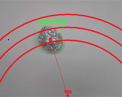
The camera wasn’t perfectly attached on the robotic arm and every little tilt of the camera would ruin the alignment. I also had to reprogram my robotic arm presets because I didn’t realize that the camera did not provide a wide enough angle and had a very narrow field of view causing my original presets to pick up something that wasn’t in the video feed. To calibrate the two, I first created three new presets that were in the video feed. I would then trace the circular movements of the robotic arm presets creating three circles. By drawing these circles, I can now align those circles with the video feed. This process was not straightforward because it was all trial and error. You can see an image of the three circles in the video feed below.

After calibrating and fixing any errors, I was able to get a working robot that can successfully recognize, pick up, and drop off an object in the location based on its material.

SECOND MILESTONE

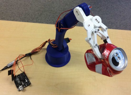
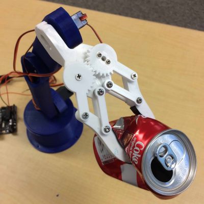
Today, I finished my second milestone which was to build and program my robotic arm. My robotic arm plays a key part in my project by picking up different recyclables and sorting them depending on its material.

The first step in completing this milestone was to get all my 3D printed parts printed and ready. Luckily, I found a predesigned 3D printed arm that I found decently compatible with my application. The 3D printed parts were printed out of a material called PLA (Polylactic Acid). It is very cheap and most well-known material for 3D printing. It is also strong enough for my project. After getting all my 3D printed parts, I had to assemble it with my servos.

I used a total of six servos. Three heavy metal geared servos and three 9 gram plastic geared servos. The three metal geared servos will be used to pivot the base of the arm and to move the lower two joints of the arm. The reason why I used metal geared servos for these parts of the arm is because those joints have to support all the weight of the arm and the object it is holding. Metal geared servos are a lot stronger and more robust than plastic geared motors due to the material of the gears. Plastic geared servos also tend to have a lower torque than metal geared servos. The only benefit is that they are much smaller and lighter. I used the 3 plastic geared servos for the top three joints of the arm including the clamping mechanism for this reason.

There were two different versions of the metal geared servo. One with high torque and one with high speed. In my project, I chose the servo with high torque, overall sacrificing the speed at which it rotates. This is done by the gear configuration in the servo. With higher torque, I can carry heavier objects. In order to control the servos of my robotic arm, I used an Arduino UNO.

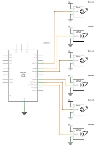
The Arduino UNO is a microcontroller that can be easily programmed on the Arduino IDE. Microcontrollers allow you to receive and transport signals to different peripherals such as sensors and in my project servos. There are three wires that come out of the servo.

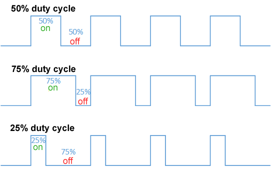
One is ground, then 5 volts, and then the signal. The 5v and ground wires are just used to power the servo motor while the signal wire is used to connect with the Arduino and control the servo. The servo can be controlled using a communication protocol called PWM, Pulse Width Modulation.

Modulation is the act of modifying or changing a frequency. In PWM it changes the width of each pulse in the digital signal. Digital signals can be thought of either on or off. Using PWM, the digital signal consists of pulses, turning on or off but at certain times. In PWM, there is something called duty cycle. Duty cycle is measured in percent of how long each pulse is in the on position. For example, a duty cycle of 70% means that the signal is 70% on and 30% off. The image below helps visualize this.

The Arduino can actually send PWM signals thanks to the built-in Servo library. With this library, all you have to do is assign the servo to a pin and set the degree at which you want it to turn to. With its pre-built functions, being able to control a servo with the Arduino is simple.

Building the robotic arm was a big challenge due to the lack of documentation on building some parts of the arm. I found it extremely difficult to build the clamping mechanism. I wasn’t sure how to construct it because I was only provided with one picture of how it should look like. I was able to use washers for the clamping mechanism joints in order to reduce friction, taking off stress from the servo. Calibrating the clamp for my servo was the next hurdle because I need to make sure that when the servo is turned all the way, the clamp would be fully closed. If I didn’t do this, the clamp would never be able to close.

After building the robotic arm, I had to wire all servos to an external power supply and connect the signal wires to the Arduino. All the 5v and ground wires of the servos were all soldered together to a 5 volt 2 amp power supply that connects to a wall outlet. I also used the power supply to power up the Arduino too. Using an external power supply, I can provide more current to all the servos than if I were to use the USB port connecting the Arduino to the computer. This also allows me to carry heavier objects. Finally, to connect the servo signal pins to the Arduino, I had to plug them into PWM capable I/O pins. There is only a selective amount of pins that can be used on the Arduino that can output PWM signals. Luckily, there are exactly six PWM pins on the Arduino.

After programming the robotic arm to move the servos in specific angles, I was able to pick up different objects and place them behind the robot. One challenge I faced was that the servos would just “snap” into position. Forcing the servo to move very fast into a specific angle while supporting the weight of the arm and the object it’s holding, putting a lot of stress on the servos that could potentially damage it. To solve this, I created a function called sweep.

Given the servo, the angle it needs to move, and the speed at which you want it to move, I can make the servo move slowly into its desired position. This is done using a for loop and a delay. The for loop will slowly increment the servo angle every few milliseconds specified in the delay function. The delay function will pause the program for a specified amount of time. Putting these together, my sweep function increments the servo angle every 15 ms. This helps the servo move a lot slower, putting less stress on the motor and gears. I’m very pleased I was able to construct my robotic arm and I look forward to moving onto my third milestone.

THIRD MILESTONE

Today I completed my first milestone which was to train an object detection model to run on the Coral Edge TPU. In my project, I trained an object detection model to distinguish between different types of recycling.

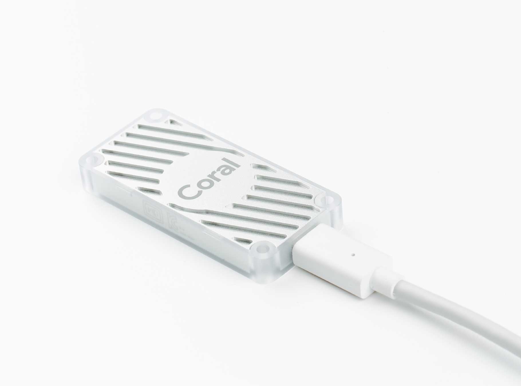
The first step in completing my first milestone was to install the Coral Edge TPU Python API on to the Raspberry Pi (RPI) in order to use my Coral USB Accelerator. The Coral Accelerator is a TPU or a tensor processing unit that you can connect to any device through a USB (universal serial bus). TPUs are processors designed specifically for machine learning purposes and thus a lot faster and more power efficient when running ML (machine learning) compared to using the RPI’s CPU. That’s why it’s called an accelerator because it accelerates the ML processing. It also includes the word “Edge” meaning all the ML processing is done locally or on the device instead of in the cloud. Using the cloud, you will need good network speed and have to pay a fee in order to use it. Using the cloud for ML is basically using someone else’s powerful TPU, CPU, or GPU to process your ML data and receiving output data via the internet. The benefits of using the Edge TPU is that you don’t need access to the internet making it a lot more versatile option. I still want to sort through recycling even if I don’t have internet access! The Edge TPU is not as powerful as the cloud solution but is suitable for my project due to the small amount of data I will be using.

After getting my RPI and Coral USB Accelerator to run a real-time object detection program using a pre-trained model, I immediately noticed how much faster the object detection was. When I tested the same model using only the RPI CPU I observed an average fps (frames per second) of 0.90. With the Coral USB Accelerator, I received an average fps of 10.40. That’s more than 11 times faster! It can process at higher rates.

There is a feature during the installation of the Coral TPU API to run the accelerator at a frequency twice the speed than the default frequency. However, there was a warning that it would get really hot and could cause burns. So I didn’t select this feature due to lack of cooling in my system. This being said, I could easily attach a small fan to cool the USB accelerator and get an fps twice as fast.

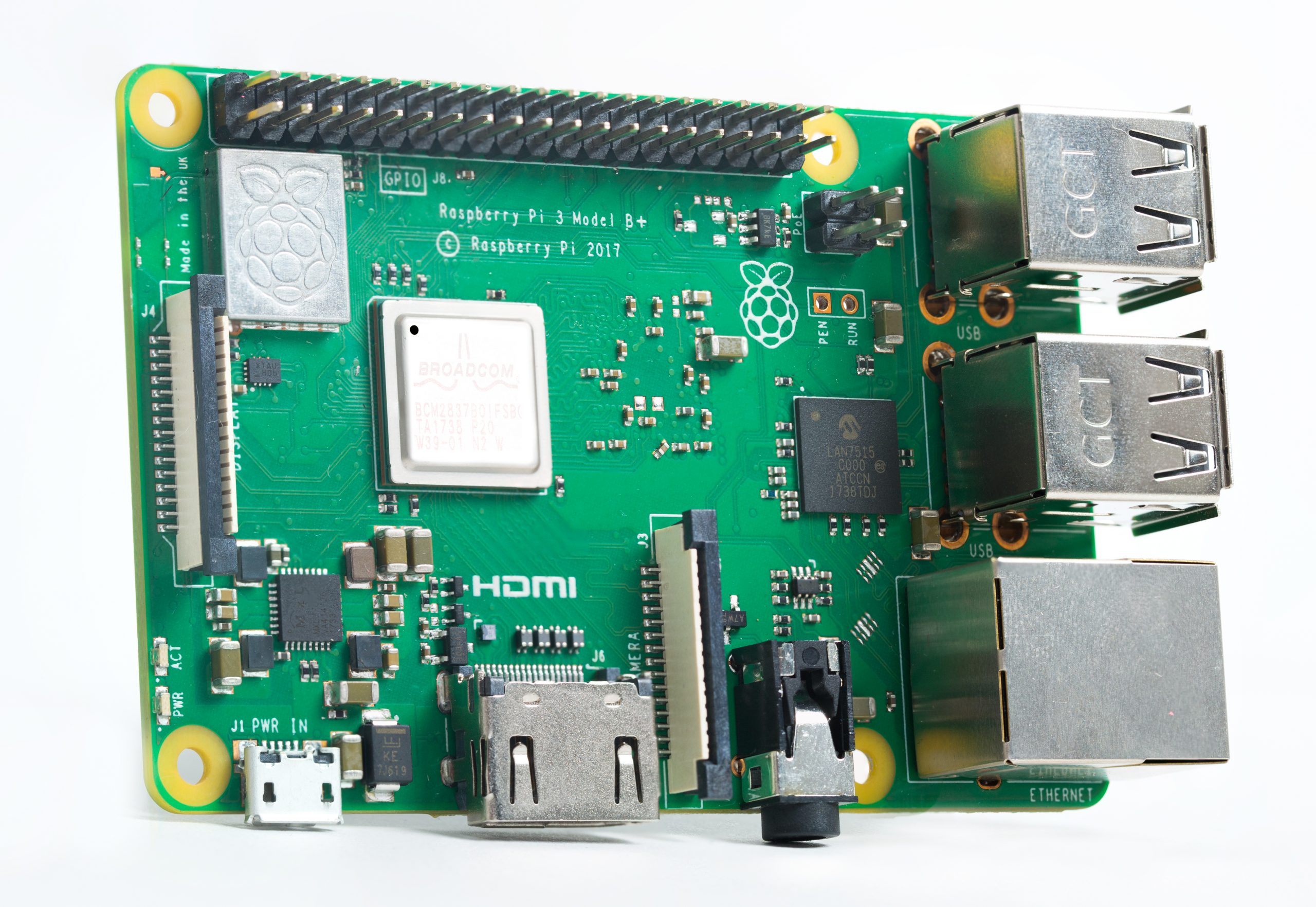
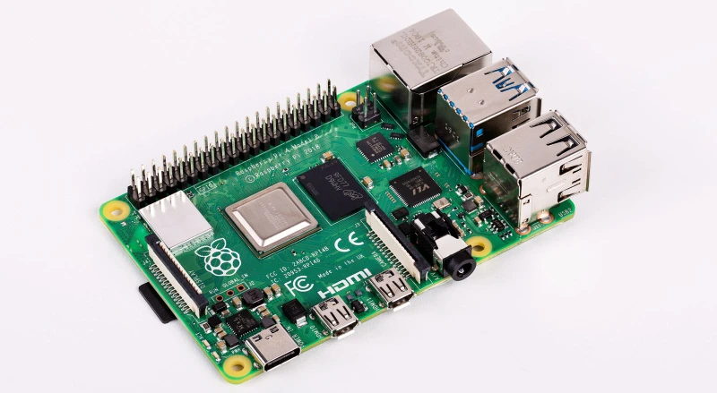
The Edge TPU also works best using USB 3 with it’s “host computer” or my RPI. Unfortunately, the RPI 3 Model B+ only has USB 2 capability, not taking full advantage of the Edge TPU’s USB 3. USB 2 transfers data at a slower rate than USB 3. This means if the RPI had USB 3 capability, I can get a faster fps due to the faster rate of data flow. Recently in June, RPI just released the RPI 4 Model B. It not only has a better CPU and RAM but also comes with USB 3 capability. Unfortunately, the Raspbian OS version is built around Python 3.7, making many of the packages I need to use for object detection incompatible. In the near future, everyone will transfer to Python 3.7, making object detection compatible with the RPI 4 Model B. Overall, taking advantage of the Edge TPU’s USB 3.

The next step would be to train my recycling model and compile it to work on the Coral Edge TPU. To explain what a model is, you can simply imagine it as the “brain” of the program. The longer you train the model, the smarter it gets. To train the model, I didn’t start from scratch. I used a technique called transfer learning.

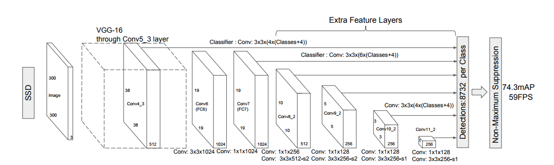
Transfer learning takes a pre-trained model and customizes it to detect certain models. This takes away all the time used to create a custom model and dealing with complicated algorithms. In my case, I used an object detection model from Tensorflow call Mobilenet v2. This model is one of the best pre-trained models out there for ML on low computational powered devices, such as my RPI or smartphones. The Mobilenet v2 runs pretty fast and is decently accurate in terms of classifying the object correctly. There are other models out there that have better accuracy, but in turn, slower to process, resulting in low fps. Using the Mobilenet v2 and transfer learning, I only changed the last few layers in the end to customize my model. Every model has tons of layers each used for a certain purpose, one to recognize each different characteristic of that object. Feeding data or in my case, a video, through those layers, you will get an output of what the model thinks it’s looking at. The image below shows how this works. I first need to collect images to create a dataset of pre-annotated images. Luckily, I found a set of images that a pair of students made during their machine learning class at Stanford with 2,500 images of different recyclables.

The set of images were made up of different materials such as paper, cardboard, glass, metal, etc. Using those images, I had to resize them to something smaller to make the training process faster by decreasing the file size. With those images, I had to annotate them. This can be done by an open source application called labelimg to simply draw a box around the object, and type in the name of that object. In my case, I had to draw boxes around pieces of paper, each labeling that it was paper. I had to repeat that for all the images and different recycling materials. After labeling, the labelimg application automatically converts them into .xml files, providing information about where the box is in the image and also the name of the object I specified. In order to train a model, you need to split your data into training and testing sets.

There are many ways to split up your data, such as 50/50, 75/25, 80/20, etc. I chose 80/20 due to the amount and diversity of my data. That means 80% of my images will go into the training set and the other 20% into the testing set. After splitting up the data, I had to convert the .xml files into .csv files so I can later convert that into a TFRecord file.

Converting the .csv files into TFRecord basically assigns a class to each object that you want to detect. In my case, I had 5 classes: cardboard, paper, metal, plastic, and glass. The TFRecord files are also the files that will be used to train my model. Now that I have a train.record and test.record file, I can now move on to creating a label map.

A label map assigns each class number with a name. For example, the first class with id: 1 is assigned the name: cardboard. After creating the label map, I can now move on to configuring the training pipeline. This can be done by changing some parameters in the pipeline.config file that came with the pre-trained model. In the pipeline.config file, I had to specify where the program can find the proper paths for my label map, TFRecord files, and my checkpoint files (comes with the pre-trained model). The checkpoint files act just like a checkpoint would in a video game. It saves progress during training. This being said, I can simply stop training, and resume it at any time. After setting up the pipeline.config file, we can now start training! You can do this in two different ways, locally or in the cloud.

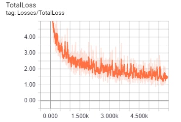
Using the cloud is a lot faster because as I stated earlier, you’re basically using someone else’s super expensive computer to do all the training. I attempted this using Google’s cloud machine learning platform but faced many errors and I decided to give up on it. So, I just trained the model locally on my laptop. This process is extremely slow and takes tons of time. As I trained the model, the program provides information about its progress and how many training steps it has completed through. Each step signifies the number of times at which the model updates its weights and biases. That is a completely different topic to explain so just think of it as each step makes the model smarter through various distinctions. More distinctions equal smarter model. In my model, I trained it around 13,000 steps. Depending on the model and the number of layers you want to retrain will affect the number of steps needed for training. Using the Mobilenet v2 model, getting a loss average below 2 is a good threshold to end training. That’s exactly what I did. You can see the graph below showing how the loss or inaccuracy of the model decreases in an exponential decay curve and ending with an average loss below 2. It’s also important to notice that the Coral Edge TPU requires an optimization technique called quantization.

This basically takes all the 32-bit floating-point numbers such as weights to the nearest 8-bit fixed-point numbers. This makes the model a lot smaller and faster without risking a significant loss in accuracy. After training the model, I then had to “freeze” it. That basically means to save the model into a protobuf file. With the .pb file you can use it to run your trained model on any CPU. However, you can’t run that model on the Coral Edge TPU. You have to convert the .pb file into a .tflite file or a tensorflow lite model.

Tensorflow lite is basically a version of Tensorflow, which is the ML library I was using, optimized for mobile usage, perfect for my RPI and the Coral USB Accelerator. In order to convert it into tensorflow lite, I needed to build TF (Tensorflow) from source. This was a lot of work! I found different tutorials about building TF from source on my laptop and kept on getting errors. I finally was able to get TF up and running by making a new Windows account because my username had a space in it, resulting in a path not found errors. I also had to do research on another bug I had with Bazel.

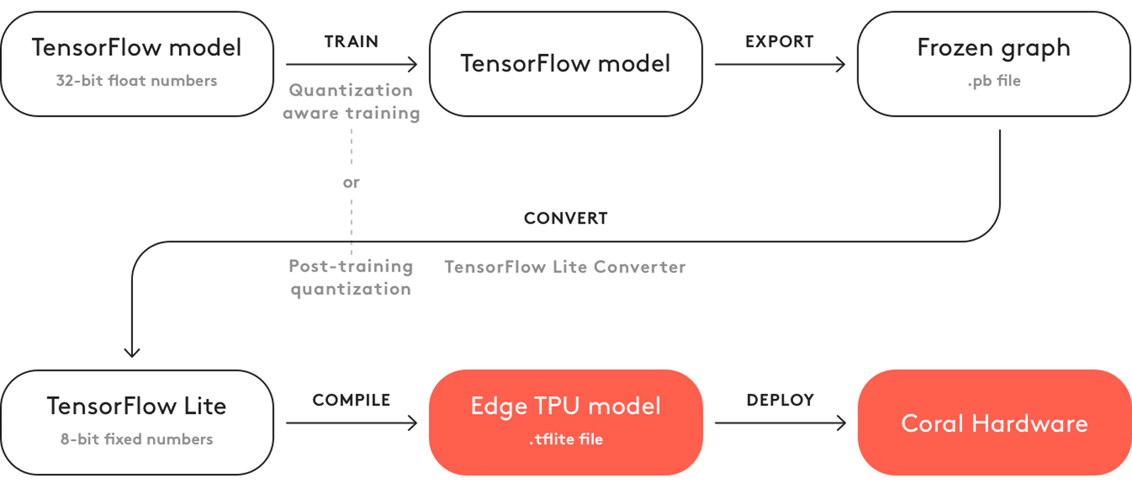
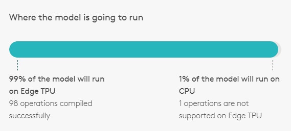
Bazel is a build tool just like make and cmake. TF wasn’t made specifically to use Bazel which lead to many errors. I finally resolved the errors and was able to use TOCO to transfer the frozen graph into a .tflite file. The final step before testing the model would be to compile the .tflite file into a model that can be used on the Coral Edge TPU. Using the Edge TPU Compiler, I compiled my .tflite another .tflite file but now compatible with the Coral USB Accelerator. As seen in the picture below, it states that 99% of the model will be run on the Edge TPU and the other 1% will run on the CPU. This takes a lot of load off of the RPI and focuses all ML processing on the Coral USB Accelerator. This leaves the RPI CPU with only a little ML processing and delivering live video feed onto the desktop. To make the process of retraining an object detection model for the Coral Edge TPU easier to understand, I included a flowchart to demonstrate the process visually.

Now that I’m done with the model, I can finally test it! Using the edge.tpu.detection.engine I can simply input my re-trained model with the live video feed to get the outputted label, confidence, and bounding box of the object that my model recognizes. This is made super easy thanks to the Edge TPU Python API. With this API, you not only can do object detection but also image classification.

Image classification simply classifies if an image includes certain objects such as a cat or dog, but doesn’t state where the object is. That is the main difference between object detection and image classification. For example, if I had a photo of a cat and used an object detection and image classification model on the same image, the object detection model will tell me that there is a cat in the image as well as where it is located, while image classification model will only tell that there is a cat in the image.

Object detection is more complicated and thus requires more computational power than image classification. In my project, I need to use object detection, so my robotic arm will know where to pick up the object according to where it is located. After using the Python API for object detection, I used the imutils module to display real-time video from the RPI camera onto the actual desktop. I also used imutils to get approximate readings of the average fps to test the efficiency of my model. Finally, I used OpenCV, which is an open source library compatible with Python, used for computer vision programs. In my case, I used it to draw information onto the desktop window. For example, I used it to draw bounding boxes around the objects my model recognizes, the corresponding name of the object, and how confident my model is about recognizing that object. Putting this all together, we can test out my model!

After starting the program I immediately faced a major issue. The model kept thinking that the whole video frame was cardboard. This happens due to two reasons, first, I had more images of cardboard than the other materials, and second, all the images were taken using a white background. Having more images of cardboard makes the model more biased to think the object is cardboard. This issue can be fixed, but I will have to take more photos of the other images to balance the number of images I have per object. For the second issue, taking all the pictures with a white background has its advantages and disadvantages. Its advantage is that it doesn’t require tons of images because all the materials will be trained on the same background, making distinguishing the object from the background easier. The disadvantage is that the model won’t be able to detect objects on a background other than white. This also can be fixed with more images with different backgrounds and lighting. However, with only 2,500 images, it’s good that all my images have the same background due to the small amount of data. The common issue I faced is lack of data.

Usually, models have hundreds of thousands of images for their model. Unfortunately, this takes a lot of time and wouldn’t be possible to complete in the time I have at BlueStamp. After the program, I will continue to add to this model to make it more accurate and more versatile by adding images with different backgrounds and lighting, as well as balancing out the number of images I have for each object. Finally, to minimize errors in my model, I simply tested out the object detection using a white background. Soon enough, it worked! There was one bug in the model that I faced even after using a white background. The model kept thinking a metallic lid was glass, not metal. This is mainly due to my labeling of images that included both metal and glass. A couple of images I used for training were glass jars that also had a metal lid on, so I made two bounding boxes around the metal and glass part of the image. This lead to the confusion of the model because sometimes the metal lid overlapped the glass jar in the image. That’s why the metal lid kept on being recognized as glass. Just like the other bugs in my model, it can be solved simply with more data. Other than that, the model performed really well with detecting different materials at different angles and lighting. I also ended up getting an average fps of 14.50. Better than the pre-trained model! This is due to the number of objects the pre-trained model could recognize compared to my re-trained model. The pre-trained model could detect 91 different objects while my model could only detect 5 different objects. Again, I could get better results if I were to use USB 3, a faster frequency on my Coral USB accelerator, and more data. Finally, I am very satisfied with the results and that I finally got it working.

Now that I’m finished with my first milestone, I will now move onto my second milestone which is to build my robotic arm.